**Note: This is a first draft of the survey, which is being submitted for review. Suggestions are most welcome.**

1 Introduction

Machine learning has become an essential part of human-machine interactions in one’s everyday life, sometimes against one’s knowledge or wish. From video-editing to voice assistants to autonomous vehicles, its benefits span a wide range of domains. Despite its seeming ubiquity, machine learning is a fast-growing research area that still faces a plethora of challenges, whether related to computational complexity [17] or data collection, among others. Among those challenges lies the rising threat of adversarial attacks [22], in which adversaries employ methods designed to take advantage of a model’s flaws for their own gain. These methods vary according to the attacker’s access to training and test data, the type of model being considered, as well as the attacker’s goal. Such attacks are particularly present in security applications like antivirus or intrusion-detection systems, but can also be found in image recognition models. Such situations can be modeled as games in which 2 or more opponents interact, with each player looking to maximize his reward while accounting for his counterpart’s actions. Adding a game-theoretic approach to the statistical modeling inherent to machine learning allows for reinforcing a model by anticipating dangerous errors, thus reducing over-fitting. This arms race between model and attacker brings an increase in security, which might come at the cost of end-user privacy, whose attempts at preserving anonymity or pseudonymity is threatened by a model’s ability to detect them.

2 Game theory and its applications

2.1 Game theory

Game theory is the study of mathematical models of strategic interaction between rational decision-makers [38]. Its growth as a discipline is attributed to von Neumann’s proof of the existence of mixed-strategy equilibria in two-person zero-sum games [41]. The theory has since been extended to n-player, cooperative or non-cooperative, zero-sum or non-zero-sum games. A fully-defined game is one that defines the following elements:

• The players

• The information available to each player

• The actions available to each player

• The payoffs for each outcome

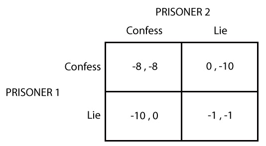
Games are represented by decision trees (extensive form), matrices (normal form) or characteristic functions. Nash [40] proved that any finite n-player, non-zero-sum, non-cooperative game has at least one equilibrium point. A Nash equilibrium is a point in the space of all possible scenarios defined by the game, where each player performs the action that maximizes his own reward according to his prediction of the action(s) of the other player(s). In such a situation, no player has any incentive to change his strategy assuming all other players are constant in their strategies. The prisoner’s dilemma (Figure 1) is a well-known two-player zero-sum, normal form game, in which two individuals are being questioned separately for a crime they are suspected of. Assuming rationality of the players, the Nash equilibrium of prisoner’s dilemma is that they will both confess, as that is the winning strategy for each player given the other’s choice, and that will not change once a player is told the other’s strategy. Notice a Nash equilibrium is optimal for each player’s individual utility: it does not necessarily maximize total social welfare.

2.2 Game theory in computing

Game theory and computer science interact in many scenarios. One the one hand, representing complex multiplayer games as well as analyzing the complexity of finding their Nash equilibria can be done through the lens of computer science: Kearn [25] provides an overview of graphical games and algorithms for finding their equilibria; Conitzer and Sandholm [7] demonstrate the algorithmic hardness of showing the existence, and the number, of a game’s Nash equilibria.

On the other hand, game theory can be a tool for finding optimal solutions to many computing problems: Koutsoupias and Papadimitriou [27] consider a noncooperative system in which players share a common resource. They propose a way of computing the cost of using the worst (in terms of social welfare) Nash equilibrium to the problem, where each player acts in his own self interest, to a socially-beneficial centralized solution. The advent of the Internet has enabled many applications that require interaction between agents. The cooperative operation of the Bitcoin [39] blockchain by miners around the world is vulnerable to attacks such as the 51% attack, where miners controlling the majority of the computing power could alter the mining process in their own selfish interest. Analysis of the decision each miner makes in cooperating or not with the system can be found in [35], [11], [23].

3 Adversarial learning

Adversarial learning consists of hardening a machine-learning model by presenting it with with inputs crafted to fool it. Traditional machine learning consists of an optimization problem, defined by a discriminative function \(f\), parameterized by a set \(\theta\), and trained to optimize a loss function \(L\) on \(n \times d\)-dimensional input data \(X\). The optimization algorithm’s goal is to find the set of parameters \(\theta^*\) that minimizes the loss with respect to the training data. Equation 1 shows a general formulation of this objective. \[\label{eq:mlobjective} \theta^* = \mathop{\mathrm{arg\,min}}_\theta \frac{1}{n} \sum_{i=1}^n L(f_\theta(x_i), x_i)\]

Once \(\theta^*\) is solved for, \(f(x)\) is measured on some test data that is separate from the training dataset. Underlying the optimization procedure is the assumption that all inputs from both the training and testing datasets are sampled independently from the same distribution. In other words, it assumes that all data points come from the same, constant, data-generating process. While the assumption holds true in many training scenarios, real-life data may show it to be overly simplistic. In many practical applications, failing to account for slightly out-of-distribution inputs can have far-reaching implications. An attacker can take advantage of this assumption in two different ways.

First, when the training data is gathered from uncontrolled sources, such as public forum posts or online images, the adversary can deliberately insert malicious examples into these sources to be picked up by the algorithm as coming from the same distribution as the rest of the data. The larger the dataset is, the more difficult it is for the modeler to notice adversarial examples.

Second, malicious examples can be fed to the model at test time to closely resemble those the model has already seen while being altered specifically to fool the algorithm, leading them to be misclassified. Cybersecurity applications, for example antivirus solutions, spam filtering and intrusion-detection systems [51], benefit particularly from adversarial learning: these systems are under constant threat of a well-crafted attack going undetected, with potentially dire consequences. For example, spyware can be hidden into innocent-looking browser toolbars, malware can be spread through peer-to-peer sharing services, and information can be stolen via malicious links in e-mail. In such a situation, the security system and its attackers are in constant learning states, where the attackers attempt to learn the detection algorithm employed by the system (in order to fool it), and the system continually improves by attempting to detect novel attacks and integrating them into the detection process.

An important step in hardening the algorithm is modeling the attacker. Huang et al. [21] decompose it into three facets: knowledge, goals and capabilities. Each factor is presented in the following subsections.

3.1 Adversarial knowledge

The attacker’s knowledge of the system will influence the design of the attacks. Three main components are identified: the algorithm, its feature space, and the training and testing datasets.

3.1.1 Knowledge of the algorithm

The attacker will hardly have perfect knowledge of the learning algorithm, unless it is publicly known or published. He can, however, anticipate the model class being used.

3.1.2 Knowledge of the feature space

Feature engineering and dimensionality reduction techniques will generally be partially or fully unknown by the attacker. Nonetheless, some domain-specific features can be common to multiple algorithms, and successful attack of one learner can lead to a better capacity of inferring some parts of the feature space.

3.1.3 Knowledge of the data

The adversary’s knowledge of the training and testing data will depend on his relationship with the target. Insiders potentially have full access to it, while foreign adversaries can get information about it. For example, https://virustotal.com acts as an online database of files scanned by the most popular antivirus solutions, as well as the classification made by each.

3.2 Adversarial capabilities

An attacker’s capabilities is closely linked to his knowledge of the target. For example, inside access to the data gives the attacker the power to alter it. Two types of influence are identified.

3.2.1 Causative influence

The attacker has the ability to alter the training data and affect the classification of specific inputs.

3.2.2 Exploratory influence

The attacker cannot alter the algorithm’s training data, but can test the system in order to gather information about its data.

3.3 Adversarial goals

The attack will be defined by the adversary’s final objective, which depends largely on the type of target and the information that it could expose. This objective is composed of the security violation desired and specificity of the attack.

3.3.1 Security violation

The attacker can target the integrity of the application, leading to false negatives being output by the classifier, or its availability, leading to false negatives and false positives and rendering the classifier unusable. He can alternatively target the application’s privacy by learning some information from the system and potentially gathering private data about its users.

3.3.2 Specificity

A targeted attack will be aimed at specific data points (e.g. classifying malicious popups as safe), while an indiscriminate one will have a broader objective (e.g. misclassifying items of any class).

4 Adversarial learning as a game

In a game of adversarial learning, the players are well defined: the learner represents one side of the game, while its attacker(s) represent the opposing side. The information available to each can be modeled using the characteristics described in section 3. What remains is to define the actions they may take as well as their payoffs. In order to do this, we need to define the playing situation. This section presents two such situations: sequential games and simultaneous games.

4.1 Sequential game

In a sequential or Stackelberg game, a leader starts by making the first move. His follower then makes his move, with full knowledge of the leader’s strategy. In such a game, each player has an advantage. The follower’s is obvious: he can observe the leader’s move and decide on his own best strategy. In other words, he does not need to model the game as a function of the leader’s action: the leader has already acted and the follower’s possible moves and their payoffs are known. The leader also benefits: by acting first, he effectively dictates the game to his opponent, restraining his actions in order to maximize his own reward. As Stackelberg games are considered constant-sum games, this strategy leads to a minimization of the follower’s reward. Research has been done modeling adversarial learning as such games, with the learner either as the leader or the follower.

4.1.1 Learner as the follower

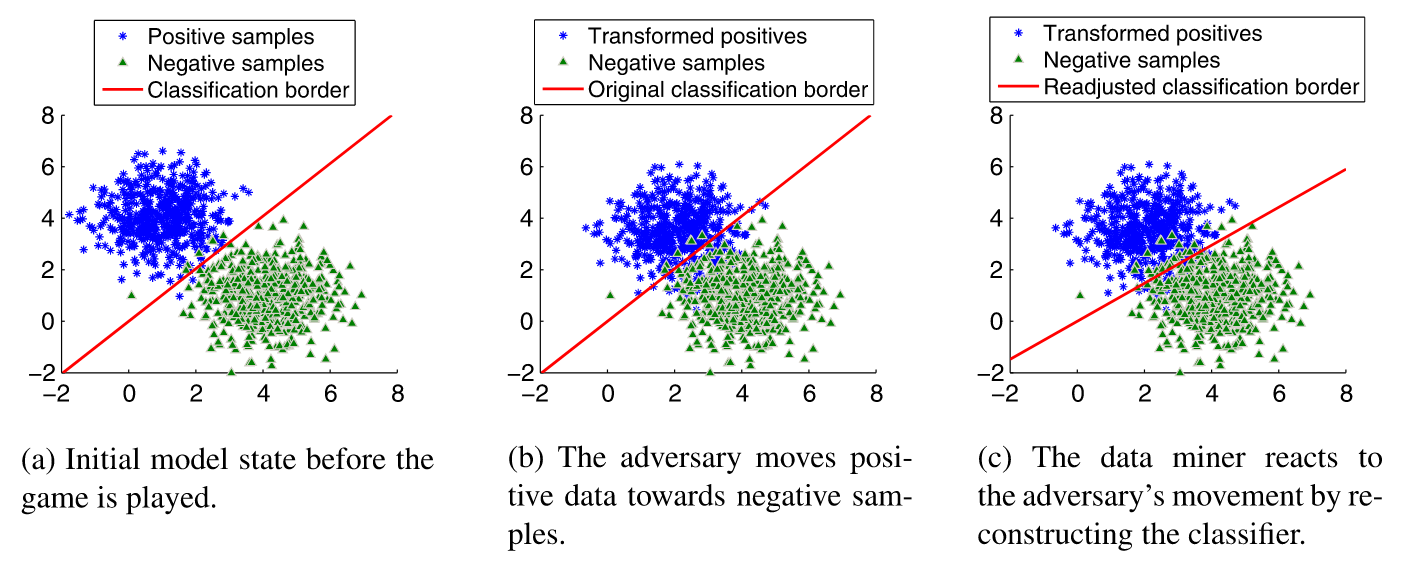
Liu and Chawla [34] propose a game where the attacker is the leader, and a classifier retroactively defends itself against an attack once it has been detected. They pose the following restriction: the classifier’s loss function must be convex and sub-differentiable: deep neural networks, whose optimization is often non-convex, are not considered valid in this setting. In this game, a binary classifier is tested by an adversary by receiving linearly-shifted inputs, which get misclassified by the learner. Upon detection of its error, the learner then learns to adjust its decision boundary to account for these new examples. Figure 2 shows an example of a linear classifier playing one round of such a game. In their example, the payoff function of the adversary corresponds to the learner’s loss function, corresponding to the negative of the classifier’s payoff. In other words:

\[\label{eq:liu2010} J_A(\alpha) = -J_C(\theta) = L(f_\theta(x_i), x_i + \alpha)\]

where \(J\) is a payoff function, \(\alpha\) is the shift applied to the inputs by the adversary \(A\), and \(\theta\) is the set of parameters of the classifier \(C\).

This leads to a zero-sum game with a Nash equilibrium where the learner’s weights and the adversary’s data manipulations have no incentive to change.

4.1.2 Learner as the leader

In some games, such as in cybersecurity systems, waiting for malicious inputs in order to adjust its parameters is too costly for the learner. In these cases, the learner is pre-trained on large amounts of data before being made available to the attacker. Its parameters are therefore fixed and available to the attacker through inference. The attacker then tries to learn these parameters by trying different input transformations and getting the learner’s classification. Spam filters are examples of such games. Brückner and Scheffer [5] formulate the optimization problem and its resulting solution as a Stackelberg prediction game using different classifier loss functions.

The games considered so far assume the adversary has but one way to transform inputs. It is also possible for an adversary to have multiple tools at his disposal: we model such a game as a multi-follower game. Zhou and Kantarcioglu [56] present a game in which a learner is opposed to multiple independent adversaries, with data transformations of varying types and degrees. They propose a framework consisting of many different Stackelberg games, each of which places a predictive model against one of the adversaries. The optimal equilibrium strategies for each of these games are used by a Bayesian Stackelberg game in which each of their classifiers is assigned a probability of being used by the learner. The added randomness makes it more difficult for the adversaries to infer the classifier’s parameters: they must now first infer the classifier chosen, and then learn its parameters.

4.2 Simultaneous game

In simultaneous games such as the prisoner’s dilemma (Figure 1), players must pick their strategy without knowing what their opponent have chosen. They simultaneously pick the action that optimizes their payoff as a function of the other player’s action. Extensive research has been done on this topic, particularly in the case of adversary feature modification or deletion. In such an attack, the adversary removes or alters features that were available during training from test inputs (by setting them to zero).

Brückner and Scheffer [4] explore simultaneous non-zero-sum games to identify conditions for determining the existence of a (unique) Nash equilibrium, which then allows to find the classifier corresponding to the equilibrium state.

Dekel, Shamir and Xiao [8] analyze the learning procedure of a binary classifier exposed to such a test-time threat. The game is formulated first as a linear programming exercise, and then as training of a modified Perceptron [48]. Globerson and Rowels [14] show, through quadratic programming, how to construct classifiers such as support vector machines that are robust to feature deletion.

Zhou et al. [57] present different optimal learner strategies based on attack models. In a free-range attack, the adversary could make any modification to any dimension of the input data. This assumes complete power of the adversary to test the learner on transformations of all kinds. In a restrained attack, the adversary is predicted to be rational, meaning his possible actions are limited to those that increase his payoff. Such transformations are generally small, with the goal of transforming an input just enough to fool the classifier. This restriction reduces the number of false positives reported by the classifier on real-life datasets in comparison to the free-range attack.

4.3 GANs

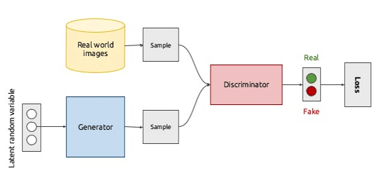
Generative adversarial networks [16] are today’s most prominent example of game-theoretic learning. Such models are in fact a pair of opposed models: a discriminator \(D\), corresponding to a binary classifier; and a generator \(G\), consisting of an unsupervised neural network attempting to learn the distribution of inputs that the discriminator classifies as positive. The setting is as follows: starting with a dataset \(X\) of inputs (typically images), \(G\) samples random noise from a distribution \(z\) to try to produce new inputs that are statistically similar to the ones from \(X\). Inputs are fed from either \(X\) or \(G\), at random, to \(D\), which is tasked with predicting whether the input is real or generated. Both models are trained simultaneously: \(D\) to learn to recognize real inputs; \(G\) to learn to generate realistic inputs. Figure 3 shows a visual representation of the training procedure.

Formally, GAN training consists of a zero-sum game with \(D\) and \(G\) as the player, and the following minimax objective: \[\label{eq:gan-objective} \arg \min_{\theta^{(G)}} \max_{\theta^{(D)}} \mathbf{E}_{x \sim \mathbf{P}_r} [\log(D(x)] + \mathbf{E}_{z \sim \mathbf{p(z)}} [\log(1 - D(G(z)]\]

Training runs until \(D\) is unable to distinguish \(G(z)\) from \(X\). In other words, convergence is achieved when \(D\) consistently makes predictions with 50% confidence. At that point, the algorithm has produced a generator capable of producing realistic inputs, as well as a strong classifier that can be reused in other scenarios.

GANs, as proposed in the original paper, are affected by a few problems. First, training is unstable and may never converge. In such a case, \(D\) and \(G\)’s payoffs are constantly oscillating without improving significantly and have to be re-initialized. Second, they are vulnerable to mode collapse, which is a state in which \(G\) has found one or a few inputs that fool \(D\), and consistently produces inputs extremely similar to them, leading to very little variety in the generated examples. Third, measuring \(G\)’s performance is very difficult: researchers often resort to manually inspecting the realism of the generated examples.

Since the publication of the original paper, GANs have been one of the most intensely-researched subject areas in the machine learning literature. Work has been done notably to improve the realism of data output by the generator, as well as to stabilize the training procedure.

4.3.1 Wasserstein GAN

Arjovsky et al. [2] propose the use of the Wasserstein distance as a replacement for the KL-divergence in the objective function of the original GAN. This improvement lead to fewer mode collapses and more stable learning. Their paper also provides ways to measure the model’s performance as it’s being trained, for quicker optimization and debugging.

4.3.2 Deep Convolutional GAN

Radford et al. [46] propose the use of convolutional neural networks [31] in the generator and discriminator for image generation tasks. CNNs are the standard in supervised image classification, but had not been previously used in unsupervised tasks such as image generation. In this paper, the authors show the superiority of convolutional generative adversarial networks in comparison to traditional feed-forward neural networks.

4.3.3 Applications to various domains

4.3.3.1 Image-to-image translation

GANs have been improved and used in a number of contexts. Zhu et al. [58] have developed an adversarial approach to image-to-image translation, which consists of learning the relationship between two images from different domains (e.g. a photograph and a painting of the same subject). The novelty of their approach is that it does not need paired images in the training data in order to learn their relationship.

4.3.3.2 Image upsampling

Most deep-learning algorithms trained for image-recognition or generation tasks work with relatively small images (typically 64x64 pixels). While the images are suitable from a learning perspective, one may need larger resolutions of the image for presentation purposes. Ledig et al. [32] propose a generative adversarial network capable of extracting the structure of an image in order to enlarge it by a factor of up to 4. They accomplish this by introducing a loss that is composed of an adversarial loss and a content loss. The adversarial loss allows the discriminator to test its ability to distinguish original images from the ones that were first upsampled by the generator. The content loss measures the loss of detail, such as high pixellation, that occurred after resizing the image.

4.3.3.3 Realistic image generation

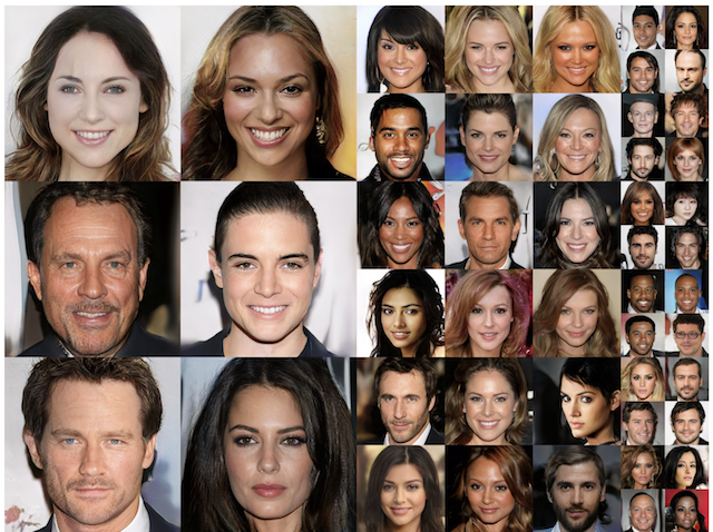
Unsurprisingly, much of the research in GANs has been made to push its limits and allow it to generate as realistic a picture as possible. Karras et al. [24] propose a GAN architecture allowing for style transfer of images, and able to generate highly-realistic faces. Some of its outputs are shown in Figure 4.

Park et al. [45] have deployed a generative model capable of creating images from a semantic sketch delimiting the various elements to be drawn (e.g. trees, water, sky).

5 Adversarial attacks and defenses

Adversarial attacks are another highly-researched application of adversarial learning. In this section, we present common attacks employed by adversaries depending on their level of knowledge of the learner and the tools at their disposal. We find three major types of attacks: evasion, poisoning, and exploratory attacks.

5.1 Evasion attacks

Evasion attacks consist of test-time generation of corrupted input data, crafted to be misclassified by the learner. In such attacks, the adversary has no ability to affect model training. Papernot et al. [44] formulate the adversary’s attack strategy as a two-step iterative method consisting of first finding the input dimensions that most affect a change in the classifier’s prediction, and second to evaluate the model based on an input transformed in these dimensions. The goal is to produce a transformation as small as possible to be misclassified by the model, while being imperceivable to a human observer. Common methods for performing the first step are presented here:

5.1.1 Fast Gradient Sign Method

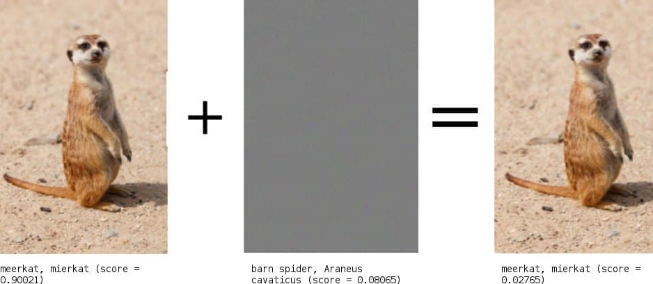
Proposed by Goodfellow et al. [15], this method alters the inputs by adding a perturbation equal to the sign of the gradient of the classifier’s loss function, scaled by a factor \(\epsilon\). In other words: \[x = x + \epsilon \cdot \text{sign}\left(\nabla_X L(x, y)\right)\] where \(y\) is the true label assigned to \(x\). This can lead to a classifier predicting the wrong class with a high confidence, as shown in Figure 5.

Two variants of FGSM have been suggested, both by Kurakin, Goodfellow and Bengio:

5.1.1.1 Target class method

Similar to the original FGSM, this method [29] however tries to fool the classifier into predicting a specific class \(y_t\). The optimization resembles the original FSGM, but replaces the true label \(y\) with \(y_t\) in the objective function.

5.1.1.2 Basic Iterative Method

In this extension [28] of FGSM, the authors suggest to iteratively modify \(x\) using element-wise clipping and show it to be able to fool smartphone cameras.

5.1.2 DeepFool

Similar to the basic iterative method, DeepFool [37] gradually perturbs inputs in order to have the learner (a deep neural network) misclassify them. The algorithm modifies the original image by moving in the direction of the loss function’s gradient (rather than its sign, as in FGSM) by projecting the example onto the learner’s decision boundary, and gets the class prediction from the label. The algorithm runs until the predicted class changes.

5.1.3 Jacobian saliency map

Papernot et al. [43] provide a more direct approach to finding the sensitivity of the classifier to input dimensions. They propose to calculate the Jacobian of the classifier’s objective function in order to obtain the gradients of each possible class with respect to the input’s dimensions. They then modify only the smallest subset of the input’s dimensions that allows for effectively fooling the learner.

5.1.4 Carlini-Wagner attack

Carlini and Wagner [6] formulate the adversarial generation objective as trying to find the smallest possible change \(\delta\) that will lead the learner to misclassify an example \(x\) with high confidence. The objective is formalized as the following: \[\delta^* = \mathop{\mathrm{arg\,min}}_\delta D(x, x + \delta) + c \cdot f(x + \delta), s.t. x + \delta \in [0, 1]^n\] where \(D\) is a distance metric between the original and perturbed examples, \(c\) is a constant scaling factor and \(f\) is an objective function such as the cross-entropy loss. They also constrain the search space of \(\delta\) by forcing the algorithm to generate valid pixel values, i.e. from 0 to 1. They test their attack on the MNIST and CIFAR-10 datasets using each of the \(L_2, L_0\) and \(L_\infty\) distances for \(D\) and 6 different objective functions for \(f\). Their attack method was able to achieve near-perfect (over 99%) misclassification on CIFAR-10, but the algorithm is computationally expensive.

5.1.5 GAN-based attacks

The generator of GANs can also be used for evasion attacks. The game setting involves a pretrained black-box discriminator \(D\), which the generator \(G\) will try to fool. GANs can be an effective adversarial tool when trained properly, and a simple pass through the generator network provides a more efficient generation process than the Carlini-Wagner attack. Bose and Aarabi [3] propose a white-box approach to generating adversarial examples for pretrained state-of-the-art Faster R-CNN [47] models. Their optimization function takes inspiration from the Carlini-Wagner formulation, and produces examples at a much higher rate. However, their method is limited to Faster R-CNN face detection classifiers, and therefore requires the adversary to know which learner class he is confronted to. Hu and Tan [20] apply GAN-based attacks to malware-detection systems. Their attack assumes the adversary has knowledge of the features used by the detection system (e.g. whether or not the example has the ability to write files to the computer).

5.2 Game-theoretic analysis

Oh et al. [42] model privacy protection as a game between a user \(U\) and a recogniser \(R\). In adversarial-learning terms, the user can be viewed as the attacker, whereas the recogniser is the learner. Neither player knows their opponent’s chosen strategy, but they are aware of his strategy space: \(\Omega^U\) and \(\Omega^R\) for the user and recognizer, respectively. \(R\)’s payoff is defined by \(p_{ij}\), corresponding to its accuracy rate for a tuble of strategies (\(i \in \Omega^U, j \in \Omega^R\)), while \(U\)’s payoff corresponds to \(R\)’s misclassification rate, and is therefore equal to \(1 - p_{ij}\). We consider this a 2-player game with a constant sum of 1. Each player can use a mixed strategy, in which his chosen strategy will be sampled randomly from a distribution \(\theta\) over his strategy space. \(U\)’s optimal mixed strategy distribution can be found by optimising the following minimax objective: \[\theta^* = \mathop{\mathrm{arg\,min}}_{\theta^U} \max_{\theta^O} \sum_{i,j} \theta^U \theta^O p_{ij}\]

Playing this optimal strategy then guarantees \(U\) a certain level of privacy (corresponding to \(R\)’s misclassification rate), regardless of \(R\)’s action. The user will use additive evasion attacks such as FGSM (subsection 5.1.1) to accomplish as high as misclassification as he can. The authors apply their methodology to a face-recognition task on 4 highly-accurate CNN architectures with various Adversarial Image Perturbation Strategies (AIPs).

5.3 Poisoning attacks

In poisoning attacks, the adversary slips infected inputs into the learner’s training data, while assigning them to a desired class. The classifier effectively learns to be misled by such examples. Those inputs can then be passed to the model at test time and should not be detected as malicious.

Such attacks can be particularly harmful in collaborative systems, such as collaborative filtering and recommender systems. Li et al. [33] present attacks to the availability and integrity of such a system, as well as a mixed strategy.

Anomaly detection systems are another vital example of binary classification tasks. Poisoning such a system has potentially serious security implications. Kloft et al. [26] solve for the optimal poisoning attack on an online centroid anomaly detection, and analyze its impact.

5.3.1 Black-box attacks through transferability

The methods presented above assumed some knowledge of the learner: either its model class, training distribution or parameter set (or a combination of those). However, in the many cases where no information is available about the learner, it is still possible to use those attacks by training a similar model on another dataset, and use the transferability property of machine learning models to attack the original target. Tramèr et al. [53] show that highly-dimensional adversarial examples share subspaces and that different models share similar directions in their decision boundaries, allowing adversarial inputs to have similar effects on multiple different models.

5.4 Exploratory attacks

As their name implies, exploratory attacks are used by adversaries with an exploratory influence on the target. They consist of inferring the state of the learner by iteratively providing examples that the adversary thinks are likely to be misclassified.

5.4.1 Model inversion

Fredrikson et al. [12] develop model inversion attacks in which an attacker can query a black-box model for prediction on an example, and receive confidence values for that input. Their technique also allows for recovering the training data used by the learner with reasonable accuracy. For example, they are able to regenerate training images used by a facial recognition API, by knowing only a person’s name and querying the model for predictions. They test their technique using a softmax regression model, a stacked denoising autoencoder and a multi-layer perceptron.

5.4.2 Model extraction

Model extraction attacks, as introduced by Tramèr et al. [54], consist of learning the black-box learner for which they only have query access to the predictions (and possibly its confidence values). In other words, their goal is to reproduce the model. This has repercussions particularly in machine-learning-as-a-service systems - where customers pay to get predictions on their data from a capable pre-trained model - as this would allow a successful adversary to resell the model as his own, or publish it for free. The authors test their attacks on two popular such services offered by Google and Amazon, for many model classes including decision trees, neural networks and logistic regression.

5.4.3 Membership inference

Shokri et al. [52] propose membership inference attacks, in which the adversary’s objective is to determine the model’s training dataset. To do so, the adversary passes examples to an online prediction API and gets its predictions. They use those results to build shadow models designed to replicate the target. Since the training and testing data for their shadow models is known, they build an attack model which compares the target’s predictions for examples that are in the shadow training set to examples that are not. This has privacy implications for sensitive datasets e.g. in the healthcare sector, where a successful adversary could gather patients’ information. The authors try their attacks on Amazon and Google’s prediction APIs.

5.5 Adversarial defenses

Protection against adversarial attacks is necessary, though difficult and impractical for two main reasons: first, anticipating adversarial attacks is a difficult task, as their attack vectors and their influences vary wildly; second, devoting too much of the model’s capacity to detecting and stopping attacks could reduce its ability to perform its predictions on non-adversarial examples, which is its primary objective. Furthermore, current defense mechanisms are typically tailored to a specific attack, so complete protection has performance drawbacks and requires longer training. This subsection explores current defense mechanisms.

5.5.1 Adversarial training

In adversarial training, the modeler transforms the training data using one of the attacks available to adversaries as a data augmentation technique. In doing so, the learner is forced to recognize these modified examples as belonging to the class of the original version, therefore preventing an adversary from successfully performing the same attack at test time. Shaham et al. [50] present a general framework in which adversarial examples are generated at each update of the learner’s parameters, providing more stable predictions and increasing the difficulty of generating adversarial examples.

5.5.2 Defensive Distillation

Distillation [18] is a technique for combining an ensemble of machine-learning models into one larger model. It consists of using the probability vectors output by an ensemble of neural networks as training labels for a smaller network (rather than the typical onehot-encoded labels), allowing for reduced complexity of the model and increased prediction speed. Papernot et al. [44] employ distillation as a hardening mechanism for the learner. The idea behind it is that adversarially-altered examples, which closely resemble their original versions, should get similar probability vectors output by the model. Therefore, crafting examples lying on a boundary between classes becomes more difficult as the labels are now softened into real numbers in the [0, 1] range, rather than binaries.

5.5.3 NULL labeling

While the mechanisms above are effective for adversarial examples generated on the learner model, they do not account for the transferability property of the examples, i.e. the adversary’s ability to generate examples for another similar model, and transfer them to the target with efficacy. To prevent transferability, Hosseini et al. [19] suggest adding an addtional class to the learner’s probability vector. The NULL class, rather than attempting to correctly classify an adversarial example using the same label as the original example, labels attacks as such by simply refusing to classify them. The training is first performed on the original dataset, after which the adversarial examples are assigned a NULL probability, which depends on their amount of corruption. The classifier is finally put through an adversarial training phase with the original and transformed examples, and is expected to assign high NULL probability to the altered inputs.

6 Privacy-conscious learning

While attack prevention is a strong research area, a lot of work is being devoted to avoiding information leakage in the eventuality of an adversarial attack. Privacy-preserving learning deals with data pre-processing and training procedures aimed at containing little-to-no private information about the training data. This is particularly critical in sensitive datasets in the healthcare industry, or confidential business datasets. We present the directions current research is taking towards private learning systems.

6.1 Noisy preprocessing

One technique for obfuscating private data is applying noise to it before feeding it to the model.

6.1.1 Adding Gaussian noise

A simple method are for adding noise to the dataset involves linearly transforming the data points. First, Domingo-Ferrer et al. [9] show how one can add random noise to the inputs \(X\) through the following transformation: \[X^{'} = X + \epsilon, \quad \epsilon \sim N(0, \Sigma_\epsilon = \alpha\Sigma)\] where \(\Sigma\) is the covariance matrix of the original dataset and \(\alpha\) is ratio of the variance of \(X^{'}\) compared to \(X\). This method preserves the mean, as well as the correlations between the input dimensions. Furthermore, it ensures that the covariance matrix of \(X^{'}\) is proportional to that of \(X\), since: \[\Sigma_{X^{'}} = \Sigma + \Sigma_\epsilon = \Sigma + \alpha \Sigma = (1 + \alpha) \cdot \Sigma\]

6.1.2 Encrypting the data

Gilad-Bachrach et al. [13] propose CryptoNets, which allow a pretrained model to make predictions based on encrypted data. The training procedure is therefore the same as with regular data, with no additional preprocessing needed. Test data is then encrypted homomorphically in order to maintain its structure. This encryption scheme allows the pretrained neural network to propagate the inputs forward through its activation layers and output a prediction as if it were dealing with the original examples. Their encryption mechanism is efficient enough to output over 59000 predictions per hour on the MNIST dataset of handwritten digits [30] despite the encryption process, but still carries an overhead when compared to training on the plain, unencrypted inputs. This method enables the user to get predictions from pretrained online machine-learning APIs without ever sending their unencrypted data through the Internet.

6.1.3 Using Garbled Circuits

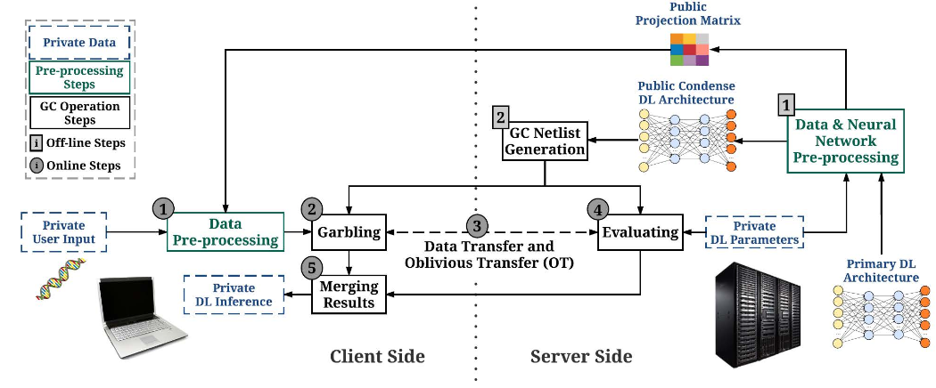
Rouhani et al. [49] provide a secure deep learning framework, named DeepSecure, for making predictions without sharing any information between parties. The authors first perform dimensionality reduction on the original input by projecting it to an ensemble of subspaces. This data is then garbled through the use of Garbled Circuits [55] and sent to the server-side learner. The learner evaluates the garbled circuit and returns its prediction based on the encrypted data. The client can then decrypt the prediction using the keys only he has access to, to get the actual predicted label associated to the original input. Figure 6 provides a visual representation of the process.

6.2 Distributing the training

Federated learning [36] is a novel approach which allows a machine-learning model to be trained without ever accessing user data. Instead of sending their private data, users only send back model-update data to a central cloud server. The process is the following: A model is first initialized by its owner, and optionally pre-trained on a large dataset (if available). The owner then connects to remote devices randomly selected from a pool of devices declaring themselves as eligible for training (McMahan el al. classify a device as eligible if it is idle and connected to a power source and an unmetered network.) The chosen devices then receive the current model, train it on their local data, and send back only the gradient of the model’s loss function. Once the owner has received a large number of these gradients, it updates its parameters using the average gradient (weighted by each user’s number of training inputs). The updated model is then sent back to users for local use or further training.

This training method effectively removes the need for a relationship between the owner of the model and the owner of the data. However, it suffers from two main drawbacks: first, the training speed will be bottlenecked by each user’s connection to the owner; second, the distribution (and number) of inputs may be very different from one user to another, which could lead the model to be trained on unbalanced or non-representative data.

6.2.1 Differential privacy

Differential privacy [10] is a method used primarily in statistical databases, where it is used as a query-time procedure that provides randomized answers to aggregation queries, that are similar to the answers one would get from the original dataset. The general goal of differential privacy is to prevent someone from telling whether a particular example is present in a dataset. Abadi et al. [1] propose a differentially-private extension of the classical SGD algorithm for model training, which applies differential privacy to the learner’s training dataset. In their extension, the training loop has two additional steps: first, the gradient of the loss function is clipped by a factor of \(1/C\) multiplied by the the gradient’s norm (where \(C\) is a clipping threshold); second, Gaussian noise is added to the clipped gradient. This added noise translates to a small difference in the impact of each training example on the learner’s parameter update. In other words, each parameter update is differentially private with respect to the training examples. Also, at each parameter update, a privacy accountant accumulates a privacy cost: a score of 0 indicates perfect privacy but may not lead to a high-performance classifier.

7 Discussion - Current limitations

Some limitations can be found in the game-theoretic framework, as well as the current performance of adversarial learning. This section presents those limitations.

7.1 Simplifying assumptions

First, an assumption being made in the game-theoretical framework is that all players are rational and behaving in their selfish best interest. If that is not the case, the optimal strategy derived from the minimax optimization may lead to suboptimal payoffs in the real world. Second, the underlying assumptions of formalizing learning as a fully-defined game as in 5.2 are that the strategy spaces of each player, along with their associated payoffs, are finite and known by both parties. Depending on the definition of the spaces (e.g. defining a strategy as a set of real-valued parameters rather than models), those assumptions can be easily violated.

7.2 Finding and end to the game

It is reasonable to wonder whether the arms race between assailants and defendants has an end. Indeed, progress by either player benefits their opponent as well. For example, new research on successful attack techniques is often followed by research on defensive mechanisms and vice-versa, therefore creating stronger players on both sides and making the game more difficult to solve.

7.3 Domain-specific applications

Much of the research currently published on adversarial learning focuses on computer vision tasks, such as object recognition and face detection. Other areas such as natural-language processing and automated speech recognition are still lagging behind. Further work into these areas is to be expected as the field matures.

7.4 Efficient, trust-less privacy

The privacy-convenience trade-off is one data owners must deal with in the current state of adversarial learning. On the one hand, easy and efficient methods such as adding random noise are always at risk of good-enough adversarial attacks that can recover the original private information. Furthermore, they are based on a relation of trust between the data user and the prediction model, particularly when it is accessible as a black-box oracle: the user must trust that the service does not store his data in insecure ways. On the other hand, trust-less options such as those presented in sections 6.1.2, 6.1.3 and 6.2 carry a computational overhead.

8 Conclusion

Three main conclusions emerge from our overview of game-theoretic adversarial learning. First, adversarial learning enables a more appropriate view of machine-learning for certain tasks, such as image generation through generative adversarial networks, and cybersecurity. Second, privacy preservation is more prevalent than ever with the advent of cloud-based machine-learning solutions, yet is a problem that has been overlooked until recently. Third and finally, while current results are promising, adversarial learning as well as machine learning still suffer from issues such as training stability, and a full understanding of the learning setting which leads to a difficulty in expanding knowledge to new tasks or providing solid training guarantees. We expect research to continue in the directions of privacy-preserving learning as well as adversarial attacks and defenses.

References

[1] Martin Abadi, Andy Chu, Ian Goodfellow, H. Brendan McMahan, Ilya Mironov, Kunal Talwar, and Li Zhang. 2016. Deep learning with differential privacy. In Proceedings of the 2016 acm sigsac conference on computer and communications security (CCS ’16), 308–318. DOI:https://doi.org/10.1145/2976749.2978318
[2] Martin Arjovsky, Soumith Chintala, and Léon Bottou. 2017. Wasserstein GAN. arXiv e-prints (January 2017), arXiv:1701.07875. Retrieved from http://arxiv.org/abs/1701.07875
[3] A. J. Bose and P. Aarabi. 2018. Adversarial attacks on face detectors using neural net based constrained optimization. In 2018 ieee 20th international workshop on multimedia signal processing (mmsp), 1–6. DOI:https://doi.org/10.1109/MMSP.2018.8547128
[4] Michael Brückner and Tobias Scheffer. 2009. Nash equilibria of static prediction games. In Advances in neural information processing systems 22, Y. Bengio, D. Schuurmans, J. D. Lafferty, C. K. I. Williams and A. Culotta (eds.). Curran Associates, Inc., 171–179. Retrieved from http://papers.nips.cc/paper/3755-nash-equilibria-of-static-prediction-games.pdf
[5] Michael Brückner and Tobias Scheffer. 2011. Stackelberg games for adversarial prediction problems. In Proceedings of the 17th acm sigkdd international conference on knowledge discovery and data mining (KDD ’11), 547–555. DOI:https://doi.org/10.1145/2020408.2020495
[6] N. Carlini and D. Wagner. 2017. Towards evaluating the robustness of neural networks. In 2017 ieee symposium on security and privacy (sp), 39–57. DOI:https://doi.org/10.1109/SP.2017.49
[7] Vincent Conitzer and Tuomas Sandholm. 2002. Complexity Results about Nash Equilibria. arXiv e-prints (May 2002), cs/0205074. Retrieved from http://arxiv.org/abs/cs/0205074
[8] Ofer Dekel, Ohad Shamir, and Lin Xiao. 2010. Learning to classify with missing and corrupted features. Machine Learning 81, 2 (November 2010), 149–178. DOI:https://doi.org/10.1007/s10994-009-5124-8
[9] Josep Domingo-Ferrer, Francesc Sebé, and Jordi Castellà-Roca. 2004. On the security of noise addition for privacy in statistical databases. In Privacy in statistical databases, 149–161.
[10] Cynthia Dwork. 2011. Differential privacy. Encyclopedia of Cryptography and Security (2011), 338–340.
[11] Ittay Eyal. 2015. The miner’s dilemma. In 2015 ieee symposium on security and privacy, 89–103.
[12] Matt Fredrikson, Somesh Jha, and Thomas Ristenpart. 2015. Model inversion attacks that exploit confidence information and basic countermeasures. In Proceedings of the 22Nd acm sigsac conference on computer and communications security (CCS ’15), 1322–1333. DOI:https://doi.org/10.1145/2810103.2813677
[13] Ran Gilad-Bachrach, Nathan Dowlin, Kim Laine, Kristin Lauter, Michael Naehrig, and John Wernsing. 2016. Cryptonets: Applying neural networks to encrypted data with high throughput and accuracy. In International conference on machine learning, 201–210.
[14] Amir Globerson and Sam Roweis. 2006. Nightmare at test time: Robust learning by feature deletion. In Proceedings of the 23rd international conference on machine learning (ICML ’06), 353–360. DOI:https://doi.org/10.1145/1143844.1143889
[15] Ian J. Goodfellow, Jonathon Shlens, and Christian Szegedy. 2014. Explaining and Harnessing Adversarial Examples. arXiv e-prints (December 2014), arXiv:1412.6572. Retrieved from http://arxiv.org/abs/1412.6572
[16] Ian Goodfellow, Jean Pouget-Abadie, Mehdi Mirza, Bing Xu, David Warde-Farley, Sherjil Ozair, Aaron Courville, and Yoshua Bengio. 2014. Generative adversarial nets. In Advances in neural information processing systems 27, Z. Ghahramani, M. Welling, C. Cortes, N. D. Lawrence and K. Q. Weinberger (eds.). Curran Associates, Inc., 2672–2680. Retrieved from http://papers.nips.cc/paper/5423-generative-adversarial-nets.pdf
[17] Joel Hestness, Newsha Ardalani, and Gregory Diamos. 2019. Beyond human-level accuracy: Computational challenges in deep learning. In Proceedings of the 24th symposium on principles and practice of parallel programming (PPoPP ’19), 1–14. DOI:https://doi.org/10.1145/3293883.3295710
[18] Geoffrey Hinton, Oriol Vinyals, and Jeff Dean. 2015. Distilling the Knowledge in a Neural Network. arXiv e-prints (March 2015), arXiv:1503.02531. Retrieved from http://arxiv.org/abs/1503.02531
[19] Hossein Hosseini, Yize Chen, Sreeram Kannan, Baosen Zhang, and Radha Poovendran. 2017. Blocking Transferability of Adversarial Examples in Black-Box Learning Systems. arXiv e-prints (March 2017), arXiv:1703.04318. Retrieved from http://arxiv.org/abs/1703.04318
[20] Weiwei Hu and Ying Tan. 2017. Generating Adversarial Malware Examples for Black-Box Attacks Based on GAN. arXiv e-prints (February 2017), arXiv:1702.05983. Retrieved from http://arxiv.org/abs/1702.05983
[21] Ling Huang, Anthony D. Joseph, Blaine Nelson, Benjamin I. P. Rubinstein, and J. D. Tygar. 2011. Adversarial machine learning. In Proceedings of the 4th acm workshop on security and artificial intelligence (AISec ’11), 43–58. DOI:https://doi.org/10.1145/2046684.2046692
[22] Sandy Huang, Nicolas Papernot, Ian Goodfellow, Yan Duan, and Pieter Abbeel. 2017. Adversarial Attacks on Neural Network Policies. arXiv e-prints (February 2017), arXiv:1702.02284. Retrieved from http://arxiv.org/abs/1702.02284
[23] Benjamin Johnson, Aron Laszka, Jens Grossklags, Marie Vasek, and Tyler Moore. 2014. Game-theoretic analysis of ddos attacks against bitcoin mining pools. In International conference on financial cryptography and data security, 72–86.
[24] Tero Karras, Timo Aila, Samuli Laine, and Jaakko Lehtinen. 2017. Progressive Growing of GANs for Improved Quality, Stability, and Variation. arXiv e-prints (October 2017), arXiv:1710.10196. Retrieved from http://arxiv.org/abs/1710.10196
[25] Michael Kearns. 2008. Graphical games. The New Palgrave Dictionary of Economics: Volume 1–8 (2008), 2547–2549.
[26] Marius Kloft and Pavel Laskov. 2010. Online anomaly detection under adversarial impact. In Proceedings of the thirteenth international conference on artificial intelligence and statistics (Proceedings of machine learning research), 405–412. Retrieved from http://proceedings.mlr.press/v9/kloft10a.html
[27] Elias Koutsoupias and Christos Papadimitriou. 1999. Worst-case equilibria. In Proceedings of the 16th annual conference on theoretical aspects of computer science (STACS’99), 404–413. Retrieved from http://dl.acm.org/citation.cfm?id=1764891.1764944
[28] Alexey Kurakin, Ian Goodfellow, and Samy Bengio. 2016. Adversarial examples in the physical world. arXiv e-prints (July 2016), arXiv:1607.02533. Retrieved from http://arxiv.org/abs/1607.02533
[29] Alexey Kurakin, Ian Goodfellow, and Samy Bengio. 2016. Adversarial Machine Learning at Scale. arXiv e-prints (November 2016), arXiv:1611.01236. Retrieved from http://arxiv.org/abs/1611.01236
[30] Yann LeCun. 1998. The mnist database of handwritten digits. http://yann. lecun. com/exdb/mnist/ (1998).
[31] Yann LeCun, Yoshua Bengio, and others. 1995. Convolutional networks for images, speech, and time series. The handbook of brain theory and neural networks 3361, 10 (1995), 1995.
[32] Christian Ledig, Lucas Theis, Ferenc Huszar, Jose Caballero, Andrew Cunningham, Alejandro Acosta, Andrew Aitken, Alykhan Tejani, Johannes Totz, Zehan Wang, and Wenzhe Shi. 2017. Photo-realistic single image super-resolution using a generative adversarial network. In The ieee conference on computer vision and pattern recognition (cvpr).
[33] Bo Li, Yining Wang, Aarti Singh, and Yevgeniy Vorobeychik. 2016. Data poisoning attacks on factorization-based collaborative filtering. In Advances in neural information processing systems 29, D. D. Lee, M. Sugiyama, U. V. Luxburg, I. Guyon and R. Garnett (eds.). Curran Associates, Inc., 1885–1893. Retrieved from http://papers.nips.cc/paper/6142-data-poisoning-attacks-on-factorization-based-collaborative-filtering.pdf
[34] Wei Liu and Sanjay Chawla. 2010. Mining adversarial patterns via regularized loss minimization. Machine Learning 81, 1 (October 2010), 69–83. DOI:https://doi.org/10.1007/s10994-010-5199-2
[35] Loi Luu, Ratul Saha, Inian Parameshwaran, Prateek Saxena, and Aquinas Hobor. 2015. On power splitting games in distributed computation: The case of bitcoin pooled mining. In 2015 ieee 28th computer security foundations symposium, 397–411.
[36] H Brendan McMahan, Eider Moore, Daniel Ramage, Seth Hampson, and others. 2016. Communication-efficient learning of deep networks from decentralized data. arXiv preprint arXiv:1602.05629 (2016).
[37] Seyed-Mohsen Moosavi-Dezfooli, Alhussein Fawzi, and Pascal Frossard. 2016. DeepFool: A simple and accurate method to fool deep neural networks. In The ieee conference on computer vision and pattern recognition (cvpr).
[38] R. B. Myerson. 1997. Game theory: Analysis of conflict. Harvard University Press. Retrieved from https://books.google.ca/books?id=E8WQFRCsNr0C
[39] Satoshi Nakamoto and others. 2008. Bitcoin: A peer-to-peer electronic cash system. (2008).
[40] John Nash. 1951. Non-cooperative games. Annals of mathematics (1951), 286–295.
[41] J v Neumann. 1928. Zur theorie der gesellschaftsspiele. Mathematische annalen 100, 1 (1928), 295–320.
[42] S. J. Oh, M. Fritz, and B. Schiele. 2017. Adversarial image perturbation for privacy protection a game theory perspective. In 2017 ieee international conference on computer vision (iccv), 1491–1500. DOI:https://doi.org/10.1109/ICCV.2017.165
[43] N. Papernot, P. McDaniel, S. Jha, M. Fredrikson, Z. B. Celik, and A. Swami. 2016. The limitations of deep learning in adversarial settings. In 2016 ieee european symposium on security and privacy (euros p), 372–387. DOI:https://doi.org/10.1109/EuroSP.2016.36
[44] N. Papernot, P. McDaniel, X. Wu, S. Jha, and A. Swami. 2016. Distillation as a defense to adversarial perturbations against deep neural networks. In 2016 ieee symposium on security and privacy (sp), 582–597. DOI:https://doi.org/10.1109/SP.2016.41
[45] Taesung Park, Ming-Yu Liu, Ting-Chun Wang, and Jun-Yan Zhu. 2019. Semantic image synthesis with spatially-adaptive normalization. In The ieee conference on computer vision and pattern recognition (cvpr).
[46] Alec Radford, Luke Metz, and Soumith Chintala. 2015. Unsupervised Representation Learning with Deep Convolutional Generative Adversarial Networks. arXiv e-prints (November 2015), arXiv:1511.06434. Retrieved from http://arxiv.org/abs/1511.06434
[47] Shaoqing Ren, Kaiming He, Ross Girshick, and Jian Sun. 2015. Faster r-cnn: Towards real-time object detection with region proposal networks. In Advances in neural information processing systems 28, C. Cortes, N. D. Lawrence, D. D. Lee, M. Sugiyama and R. Garnett (eds.). Curran Associates, Inc., 91–99. Retrieved from http://papers.nips.cc/paper/5638-faster-r-cnn-towards-real-time-object-detection-with-region-proposal-networks.pdf
[48] Frank Rosenblatt. 1958. The perceptron: A probabilistic model for information storage and organization in the brain. Psychological review 65, 6 (1958), 386.
[49] Bita Darvish Rouhani, M. Sadegh Riazi, and Farinaz Koushanfar. 2018. Deepsecure: Scalable provably-secure deep learning. In Proceedings of the 55th annual design automation conference (DAC ’18), 2:1–2:6. DOI:https://doi.org/10.1145/3195970.3196023
[50] Uri Shaham, Yutaro Yamada, and Sahand Negahban. 2018. Understanding adversarial training: Increasing local stability of supervised models through robust optimization. Neurocomputing 307, (2018), 195–204. DOI:https://doi.org/https://doi.org/10.1016/j.neucom.2018.04.027
[51] Yue Shen, Zheng Yan, and Raimo Kantola. 2014. Analysis on the acceptance of global trust management for unwanted traffic control based on game theory. Computers & Security 47, (2014), 3–25. DOI:https://doi.org/https://doi.org/10.1016/j.cose.2014.03.010
[52] R. Shokri, M. Stronati, C. Song, and V. Shmatikov. 2017. Membership inference attacks against machine learning models. In 2017 ieee symposium on security and privacy (sp), 3–18. DOI:https://doi.org/10.1109/SP.2017.41
[53] Florian Tramèr, Nicolas Papernot, Ian Goodfellow, Dan Boneh, and Patrick McDaniel. 2017. The Space of Transferable Adversarial Examples. arXiv e-prints (April 2017), arXiv:1704.03453. Retrieved from http://arxiv.org/abs/1704.03453
[54] Florian Tramèr, Fan Zhang, Ari Juels, Michael K. Reiter, and Thomas Ristenpart. 2016. Stealing machine learning models via prediction apis. In 25th USENIX security symposium (USENIX security 16), 601–618. Retrieved from https://www.usenix.org/conference/usenixsecurity16/technical-sessions/presentation/tramer
[55] A. C. Yao. 1986. How to generate and exchange secrets. In 27th annual symposium on foundations of computer science (sfcs 1986), 162–167. DOI:https://doi.org/10.1109/SFCS.1986.25
[56] Yan Zhou and Murat Kantarcioglu. 2016. Modeling adversarial learning as nested stackelberg games. In Advances in knowledge discovery and data mining, 350–362.
[57] Yan Zhou, Murat Kantarcioglu, Bhavani Thuraisingham, and Bowei Xi. 2012. Adversarial support vector machine learning. In Proceedings of the 18th acm sigkdd international conference on knowledge discovery and data mining (KDD ’12), 1059–1067. DOI:https://doi.org/10.1145/2339530.2339697
[58] Jun-Yan Zhu, Taesung Park, Phillip Isola, and Alexei A Efros. 2017. Unpaired image-to-image translation using cycle-consistent adversarial networks. In Computer vision (iccv), 2017 ieee international conference on.